State Space Models - Discretization and Convolution

Transformers models have been at the forefront of AI development for the past couple of years. Transformer architecture utilizes the concept of self-attention, enabling the model to generate output not solely based on the input sequence but also leveraging the context between all tokens in the input sequence. This context is used as an attention matrix to produce output tokens. The success of the Transformers architecture lies in its self-attention mechanism and its ability to train the model in parallel on the input sequence, eliminating the need to process the sequence step by step.

However, a drawback of this architecture is its quadratic complexity in computing self-attention. This limitation makes it less efficient for inference with a large context window, as it requires computing the attention of all previous tokens every time to predict the next token.

To address this quadratic complexity issue, we are exploring the State Space model (SSM), which is touted to perform inference on the next token or output in constant time. SSMs are sequence models, similar to RNNs, but with the capability of parallelization.

Sequence Models

Sequence models aim to map input sequences to output sequences, These models can map both continuous data, such as audio, and discrete data, such as text to some output sequence.

RNNs (recurrent neural networks) and its variants were the popular choice for sequencing models, mainly used for language modeling before the Transformer architecture became popular. RNNs handle sequential input data through individual time steps, keeping a hidden state that acts as memory and is updated based on current input and past hidden states. By using shared weights and parameters, the network calculates outputs at each time step, allowing tasks like predicting the next element. Theoretically, RNNs have an infinite context window as they can process the input sequence indefinitely. However, they face challenges like vanishing/exploding gradients. Additionally, training this model isn’t parallelizable, as each token needs to be input one by one based on the timestamp.

Despite these issues, RNNs can perform inference at a consistent time for each token.So, we want an Architecture something like RNNs which can:

1. Parallelize the training (like the Transformer) and can scale linearly to long sequences

2. Can inference each token with a constant computation $O(1)$ (like the RNN)

State Space Models

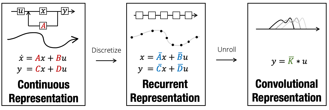
The state space model provided a systematic way to describe the dynamics of a system in terms of a set of equations that represented the ‘state’ of the system and how this state evolved over time. We usually use differential equations to model the state of a system over time, with the goal of finding a function that gives us the state of the system at any time step, given the initial state of the system at time 0.

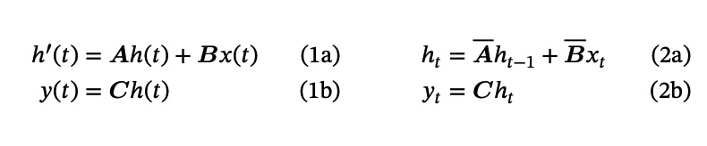
A state space model allows us to map an input signal $x(t)$ to an output signal $y(t)$ by means of a state representation $h(t)$ as follows:

This state space model is linear and time invariant. Linear because the relationships in the expressions above are linear, and time invariant because the parameter matrices A, B, C, D do not depend on time (they are fixed).

To find the output signal $y(t)$ at time $t$, we first need to find a function $h(t)$ that describes the state of the system for all time steps. But that can be hard to solve analytically.

Usually, we never work with continuous signals, but always with discrete ones (because we sample them), so how can we produce outputs $y(t)$ for a discrete signal? We first need to discretize our system!

Discretization

To solve a differential equation, we need to find the function $h(t)$ that makes the two hand sides of the equation equal, but most of the time it’s hard to find the analytical solution of a differential equation. That’s why we can approximate the solution of a differential equation. To find the approximate solution of a differential equation means to find a sequence of $h(0)$, $h(1)$, $h(2)$, $h(3)$, etc. that describe the evolution of our system over time. So instead of finding $h(t)$ we want to find $h(t_{k}) = h(k\Delta)$ where $\Delta$ is our step size.

Here we will perform discretization on an example equation $b(t)$ - using Euler’s method! ( Several methods for discretization/approximation available)

1. Let us assume differential equation for which we want to calculate 𝑏(𝑡) is like this : 𝑏’(𝑡) = 𝝀𝑏(𝑡)

2. The derivative is the rate of change of the function,we can write it as: $\lim_{\Delta \to 0} \frac{ b(t+\Delta) - b(t) }{\Delta}$ = 𝑏′(𝑡).
3. By choosing a small step size ∆ we can approximate the limit: $\frac{ b(t+\Delta) - b(t) }{\Delta}$ ≅ 𝑏′(𝑡). By multiplying with ∆ and moving terms around we can further write: 𝑏(𝑡 + ∆) ≅ 𝑏′(𝑡) ∆ + 𝑏 (𝑡)
4. We can then plug value into the previous expression to obtain: 𝑏(𝑡 + ∆) ≅ 𝝀b(𝑡)∆ + 𝑏(𝑡) a recurrent formulation!

By using a similar reasoning, we can also discretize our state space model, so that we can calculate the evolution of the state over time by using a recurrent formulation.

1. By using the definition of derivative we know that: ℎ(𝑡 + ∆) ≅ ∆ℎ′(𝑡) + ℎ(𝑡)
2. This is the (continuous) state space model: ℎ′(𝑡) = 𝑨ℎ(𝑡) + 𝑩𝑥(𝑡)
3. We can substitute the state space model into the first expression to get the following \(\begin{align*} ℎ(𝑡 + ∆) &≅ ∆( 𝑨ℎ(𝑡) + 𝑩𝑥(𝑡) ) + ℎ (𝑡)\\ &= ∆𝑨ℎ(𝑡) + ∆𝑩𝑥(𝑡) + ℎ(𝑡) \\ &= (𝐼 + ∆𝑨) ℎ(𝑡) + ∆𝑩𝑥(𝑡)\\ &= \bar Aℎ(𝑡) + \bar B𝑥(𝑡) \end{align*}\)

Now we have a recurrent formula that allows us to iteratively calculate the state of the system one step at a time, knowing the state at the previous time step. The matrices $ \bar A $ and $ \bar B $ are the discretized parameters of the model. This allows us to also calculate the output 𝑦(𝑡) of the system for discrete time steps.

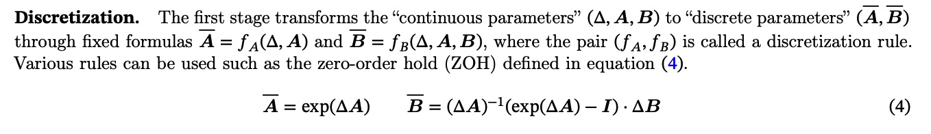
In the paper instead of the Euler method they use the Zero-Order Hold (ZOH) rule to discretize the system. Note: in practice, we do not choose the discretization step ∆, but we make it a parameter of the model so that it can be learnt with gradient descent.

Convulation: Making SSM parallelizable

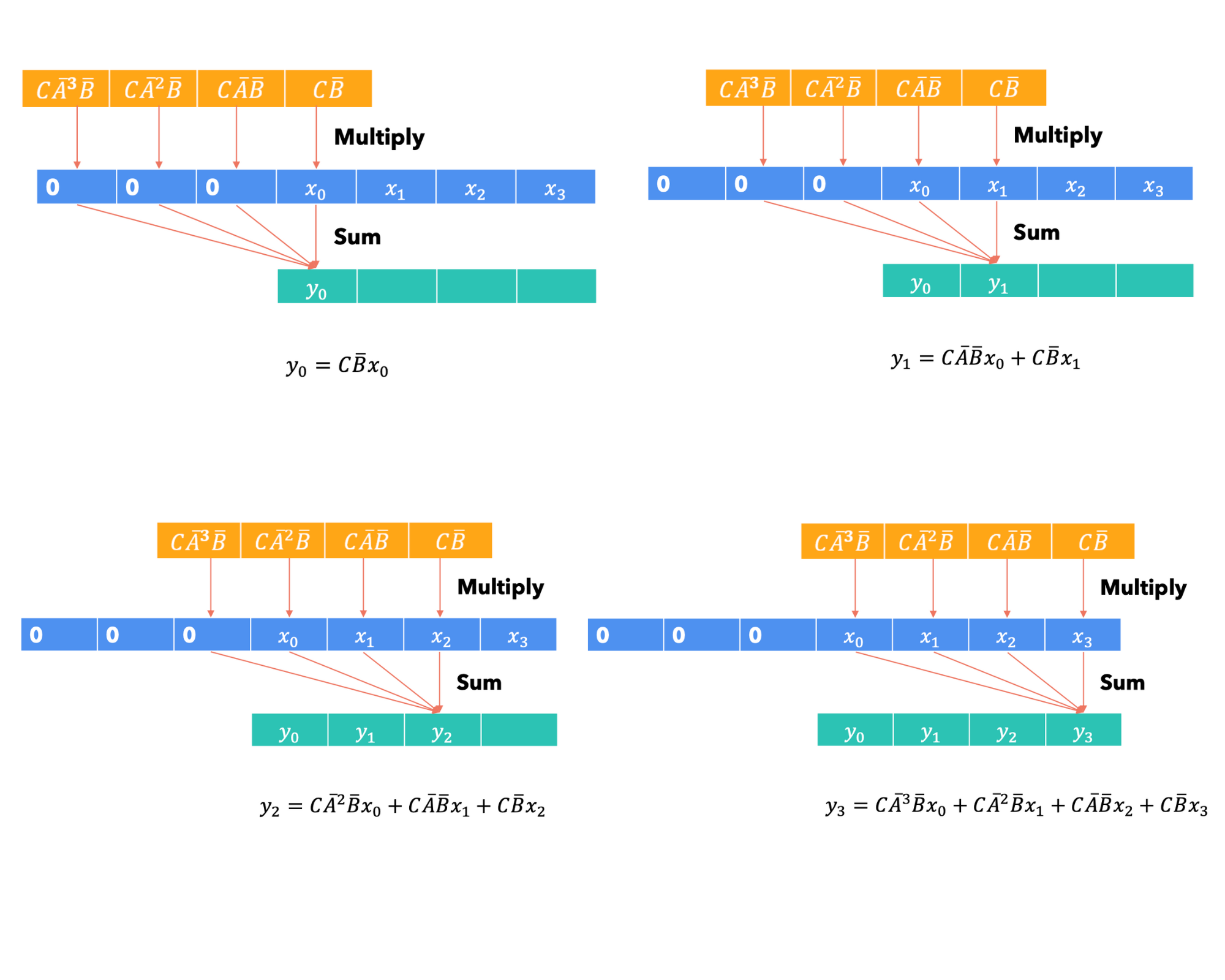
The recurrent formulation is not good for training, because during training we already have all the tokens of the input and the target, so we want to parallelize the computation as much as possible, just like the Transformer does! To convert the recurrent formula derived into convolutional view, we need to iterate over the equation, to find the general equation for our Kernel ($\mathbf{K}$):

Let’s expand these equation for each time step:

The General equation is something like:

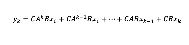
We can observe $\mathbf{\bar K}$ as the SSM convolution kernel, and its size is equivalent to the entire input sequence:

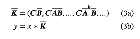
The advantage of using convolutional calculation is that it can be parallelized since the output does not depend on previous outputs. However, constructing the kernel can be computationally expensive and memory-intensive. Convolutional computation is suitable for training, as it can be parallelized with the input sequence. On the other hand, the recurrent formulation is more suitable for inference, processing one token at a time with a consistent amount of computation and memory.

References

• Efficiently Modeling Long Sequences with Structured State Spaces
• Mamba: Linear-Time Sequence Modeling with Selective State Spaces
• Blog post by Albert GU et al. (2022)
• Mamba and S4 Explained video by Umar Jamil